Tidy modelling

Readings and class materials for Tuesday, November 14, 2023

Suggested materials

Tidy Modeling with R

In the previous chapter, we observed that a machine learning tool, regardless of the chosen model, is built upon a very similar recipe. Firstly, we provide it with data, on which certain transformations may be performed beforehand. Then, we train a model on a given dataset, varying the hyperparameters, and evaluate its predictions on another dataset. Subsequently, we either utilize the model to make predictions, preferably the best ones, or examine which variable proved to be the most important based on certain metrics (we consider which approach was employed most frequently or which one significantly improved the predictive capability of the model)

As the Tidyverse contains a collection of packages that are generally useful and frequently used for reading, cleaning, and visualizing data, the tidymodels is a package collection that includes important tools for modelling, when we focus on prediction.

The tidymodels packages are designed to work together, and they are built on top of the Tidyverse. The packages are designed to be modular, so that you can easily mix and match them to suit your needs.

https://www.tidymodels.org/packages/

Let us proceed step by step…

Splitting (resamples)

data(attrition, package = "modeldata")

glimpse(attrition)

Rows: 1,470
Columns: 31
$ Age                      <int> 41, 49, 37, 33, 27, 32, 59, 30, 38, 36, 35, 2…
$ Attrition                <fct> Yes, No, Yes, No, No, No, No, No, No, No, No,…
$ BusinessTravel           <fct> Travel_Rarely, Travel_Frequently, Travel_Rare…
$ DailyRate                <int> 1102, 279, 1373, 1392, 591, 1005, 1324, 1358,…
$ Department               <fct> Sales, Research_Development, Research_Develop…
$ DistanceFromHome         <int> 1, 8, 2, 3, 2, 2, 3, 24, 23, 27, 16, 15, 26, …
$ Education                <ord> College, Below_College, College, Master, Belo…
$ EducationField           <fct> Life_Sciences, Life_Sciences, Other, Life_Sci…
$ EnvironmentSatisfaction  <ord> Medium, High, Very_High, Very_High, Low, Very…
$ Gender                   <fct> Female, Male, Male, Female, Male, Male, Femal…
$ HourlyRate               <int> 94, 61, 92, 56, 40, 79, 81, 67, 44, 94, 84, 4…
$ JobInvolvement           <ord> High, Medium, Medium, High, High, High, Very_…
$ JobLevel                 <int> 2, 2, 1, 1, 1, 1, 1, 1, 3, 2, 1, 2, 1, 1, 1, …
$ JobRole                  <fct> Sales_Executive, Research_Scientist, Laborato…
$ JobSatisfaction          <ord> Very_High, Medium, High, High, Medium, Very_H…
$ MaritalStatus            <fct> Single, Married, Single, Married, Married, Si…
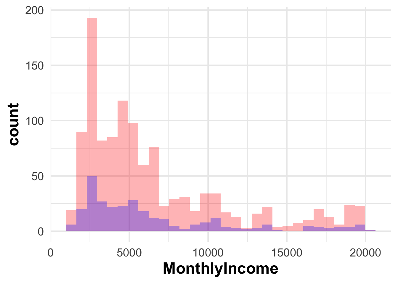
$ MonthlyIncome            <int> 5993, 5130, 2090, 2909, 3468, 3068, 2670, 269…
$ MonthlyRate              <int> 19479, 24907, 2396, 23159, 16632, 11864, 9964…
$ NumCompaniesWorked       <int> 8, 1, 6, 1, 9, 0, 4, 1, 0, 6, 0, 0, 1, 0, 5, …
$ OverTime                 <fct> Yes, No, Yes, Yes, No, No, Yes, No, No, No, N…
$ PercentSalaryHike        <int> 11, 23, 15, 11, 12, 13, 20, 22, 21, 13, 13, 1…
$ PerformanceRating        <ord> Excellent, Outstanding, Excellent, Excellent,…
$ RelationshipSatisfaction <ord> Low, Very_High, Medium, High, Very_High, High…
$ StockOptionLevel         <int> 0, 1, 0, 0, 1, 0, 3, 1, 0, 2, 1, 0, 1, 1, 0, …
$ TotalWorkingYears        <int> 8, 10, 7, 8, 6, 8, 12, 1, 10, 17, 6, 10, 5, 3…
$ TrainingTimesLastYear    <int> 0, 3, 3, 3, 3, 2, 3, 2, 2, 3, 5, 3, 1, 2, 4, …
$ WorkLifeBalance          <ord> Bad, Better, Better, Better, Better, Good, Go…
$ YearsAtCompany           <int> 6, 10, 0, 8, 2, 7, 1, 1, 9, 7, 5, 9, 5, 2, 4,…
$ YearsInCurrentRole       <int> 4, 7, 0, 7, 2, 7, 0, 0, 7, 7, 4, 5, 2, 2, 2, …
$ YearsSinceLastPromotion  <int> 0, 1, 0, 3, 2, 3, 0, 0, 1, 7, 0, 0, 4, 1, 0, …
$ YearsWithCurrManager     <int> 5, 7, 0, 0, 2, 6, 0, 0, 8, 7, 3, 8, 3, 2, 3, …

library(tidymodels)

attrition_split <- initial_split(tibble(attrition), prop = 0.8)

Once we have a cleaned dataset, we can split it into two parts. The first part is used for training the model, and the second part is used for testing the model. The initial_split() function performs this split. The prop argument specifies the proportion of the data that should be used for training. The default value is 0.75, which means that 75% of the data will be used for training and 25% for testing. This is fine in most cases. The initial_split() function returns a list containing two tibbles: the training data and the testing data.

training(attrition_split)

# A tibble: 1,176 × 31
     Age Attrition BusinessTravel    DailyRate Department       DistanceFromHome
   <int> <fct>     <fct>                 <int> <fct>                       <int>
 1    56 Yes       Travel_Rarely           310 Research_Develo…                7
 2    35 No        Travel_Rarely           672 Research_Develo…               25
 3    21 No        Travel_Rarely           501 Sales                           5
 4    33 Yes       Travel_Frequently       827 Research_Develo…               29
 5    34 No        Travel_Rarely          1351 Research_Develo…                1
 6    39 No        Travel_Rarely          1387 Research_Develo…               10
 7    38 No        Travel_Rarely          1495 Research_Develo…                4
 8    26 No        Travel_Rarely           991 Research_Develo…                6
 9    34 No        Travel_Rarely          1397 Research_Develo…                1
10    38 No        Travel_Rarely          1009 Sales                           2
# ℹ 1,166 more rows
# ℹ 25 more variables: Education <ord>, EducationField <fct>,
#   EnvironmentSatisfaction <ord>, Gender <fct>, HourlyRate <int>,
#   JobInvolvement <ord>, JobLevel <int>, JobRole <fct>, JobSatisfaction <ord>,
#   MaritalStatus <fct>, MonthlyIncome <int>, MonthlyRate <int>,
#   NumCompaniesWorked <int>, OverTime <fct>, PercentSalaryHike <int>,
#   PerformanceRating <ord>, RelationshipSatisfaction <ord>, …

testing(attrition_split)

# A tibble: 294 × 31
     Age Attrition BusinessTravel    DailyRate Department       DistanceFromHome
   <int> <fct>     <fct>                 <int> <fct>                       <int>
 1    33 No        Travel_Frequently      1392 Research_Develo…                3
 2    36 No        Travel_Rarely          1299 Research_Develo…               27
 3    31 No        Travel_Rarely           670 Research_Develo…               26
 4    29 No        Travel_Rarely          1389 Research_Develo…               21
 5    34 No        Travel_Rarely           419 Research_Develo…                7
 6    53 No        Travel_Rarely          1282 Research_Develo…                5
 7    30 No        Travel_Rarely           125 Research_Develo…                9
 8    24 Yes       Travel_Rarely           813 Research_Develo…                1
 9    43 No        Travel_Rarely          1273 Research_Develo…                2
10    27 No        Travel_Rarely          1240 Research_Develo…                2
# ℹ 284 more rows
# ℹ 25 more variables: Education <ord>, EducationField <fct>,
#   EnvironmentSatisfaction <ord>, Gender <fct>, HourlyRate <int>,
#   JobInvolvement <ord>, JobLevel <int>, JobRole <fct>, JobSatisfaction <ord>,
#   MaritalStatus <fct>, MonthlyIncome <int>, MonthlyRate <int>,
#   NumCompaniesWorked <int>, OverTime <fct>, PercentSalaryHike <int>,
#   PerformanceRating <ord>, RelationshipSatisfaction <ord>, …

In many cases, it is important that the data we use to train the model and evaluate it is similar according to certain criteria. For example, if significant differences are observed in salaries, it is important to separate the original data in such a way that the distribution of salaries is the same in the training and testing tables. This can be ensured using the strata argument.

attrition_split <- initial_split(tibble(attrition), prop = 0.8, strata = "MonthlyIncome")

ggplot() +
  aes(MonthlyIncome) +
  geom_histogram(data=training(attrition_split), alpha = .3, fill = "red") +
  geom_histogram(data=testing(attrition_split), alpha = .3, fill = "blue")

Furthermore, we have observed that each model possesses different hyperparameters. In the case of decision trees, the complexity of the tree is determined, while for other models, the number of degree of freedom terms to be applied is considered. Every other model will also have its own set of hyperparameters. We are seeking the combination of hyperparameters that yields the best performance. Typically, this is not achieved by solely evaluating the model’s performance on the test data using the training data, but by further dividing the training data. One example of this is k-fold cross-validation. In the case of k-fold cross-validation, if we divide the data into 10 parts, the model is trained on 90% of the previously created training data, and evaluated on the remaining 10% for a given set of hyperparameters. Then, we reverse the process and evaluate on another 10%. This process is repeated k (10) times. The average of the results is then calculated. This is a very common method for evaluating models. The rsample package contains a function that performs this split. The vfold_cv() function performs this split. The number of folds is specified by the v argument. The default value is 10.

attrition_vsplit <- vfold_cv(tibble(attrition), v = 10)

attrition_vsplit

#  10-fold cross-validation 
# A tibble: 10 × 2
   splits             id    
   <list>             <chr> 
 1 <split [1323/147]> Fold01
 2 <split [1323/147]> Fold02
 3 <split [1323/147]> Fold03
 4 <split [1323/147]> Fold04
 5 <split [1323/147]> Fold05
 6 <split [1323/147]> Fold06
 7 <split [1323/147]> Fold07
 8 <split [1323/147]> Fold08
 9 <split [1323/147]> Fold09
10 <split [1323/147]> Fold10

The cross-validation procedure can be very complex at times, for example when we want to forecast time series and always need to separate the data from the past five years to examine how we would forecast the next year. This can be done using the rset_manual function. This procedure is called step-forward cross-validation, and you can see an example of it in the link below. We could also mention the example of predicting stock prices or any other economic variable.

If sample size is a consideration, it may be worth choosing bootstrapping instead of simple cross-validation, as in this case the measurements of the individual training and test sets will be identical, and then randomly divide the dataset, using random sampling, to collect the samples. This enables us to run the model a very large number of times, in a very large quantity, under a given parameter, while keeping the size constant.

bootstraps(training(attrition_split), times = 100)

# Bootstrap sampling 
# A tibble: 100 × 2
   splits             id          
   <list>             <chr>       
 1 <split [1174/433]> Bootstrap001
 2 <split [1174/436]> Bootstrap002
 3 <split [1174/416]> Bootstrap003
 4 <split [1174/450]> Bootstrap004
 5 <split [1174/428]> Bootstrap005
 6 <split [1174/406]> Bootstrap006
 7 <split [1174/426]> Bootstrap007
 8 <split [1174/433]> Bootstrap008
 9 <split [1174/434]> Bootstrap009
10 <split [1174/437]> Bootstrap010
# ℹ 90 more rows

Preprocessing (recipes)

After splitting the data, it is necessary to perform transformations for certain models. Such a transformation could be, for example, standardization or excluding variables that have very high correlation or variables that have zero variabilty. Let’s assume, for example, that we have a training data in which only one type of value occurs in a certain variable. For instance, only males are present in the training data. Obviously, when we want to make predictions with this model, we will not be able to use this column. Therefore, it is necessary that during training, this column is excluded. We can imagine that we have hundreds of variables and we cannot ensure that we can always filter out these columns in the training data. For example, we run the model for each year.

The tidymodels package collection contains the recipe package that allows us to perform such transformations. The recipe package is designed to create a blueprint for a model. It is a collection of steps that will be performed on the data before the model is trained. The recipe package contains a number of functions that can be used to create a recipe. The recipe() function creates a recipe object. The step_*() functions add steps to the recipe. The prep() function prepares the recipe, and the bake() function applies the recipe to the data.

The recipe() function takes two arguments. The first argument is the formula that specifies the target variable and the explanatory variables. The second argument is the data frame that contains the data. The step_*() functions take the recipe object as the first argument and the name of the step as the second argument. The prep() function takes the recipe object as the first argument. The bake() function takes the recipe object as the first argument and the data frame as the second argument.

attrition_vsplit %>% 
  pull(splits)

[[1]]
<Analysis/Assess/Total>
<1323/147/1470>

[[2]]
<Analysis/Assess/Total>
<1323/147/1470>

[[3]]
<Analysis/Assess/Total>
<1323/147/1470>

[[4]]
<Analysis/Assess/Total>
<1323/147/1470>

[[5]]
<Analysis/Assess/Total>
<1323/147/1470>

[[6]]
<Analysis/Assess/Total>
<1323/147/1470>

[[7]]
<Analysis/Assess/Total>
<1323/147/1470>

[[8]]
<Analysis/Assess/Total>
<1323/147/1470>

[[9]]
<Analysis/Assess/Total>
<1323/147/1470>

[[10]]
<Analysis/Assess/Total>
<1323/147/1470>

attrition_recipe <- recipe(MonthlyIncome ~ ., data = attrition) %>% 
  step_rm(RelationshipSatisfaction) %>% # should use this?
  step_dummy(all_nominal()) %>%
  step_corr(all_numeric())

attrition_recipe_preped <- attrition_recipe %>% 
  prep()

attrition_vsplit %>% 
  pull(splits)

[[1]]
<Analysis/Assess/Total>
<1323/147/1470>

[[2]]
<Analysis/Assess/Total>
<1323/147/1470>

[[3]]
<Analysis/Assess/Total>
<1323/147/1470>

[[4]]
<Analysis/Assess/Total>
<1323/147/1470>

[[5]]
<Analysis/Assess/Total>
<1323/147/1470>

[[6]]
<Analysis/Assess/Total>
<1323/147/1470>

[[7]]
<Analysis/Assess/Total>
<1323/147/1470>

[[8]]
<Analysis/Assess/Total>
<1323/147/1470>

[[9]]
<Analysis/Assess/Total>
<1323/147/1470>

[[10]]
<Analysis/Assess/Total>
<1323/147/1470>

attrition_vsplit %>% 
  pull(splits) %>% 
  first() %>% 
  analysis()

# A tibble: 1,323 × 31
     Age Attrition BusinessTravel    DailyRate Department       DistanceFromHome
   <int> <fct>     <fct>                 <int> <fct>                       <int>
 1    41 Yes       Travel_Rarely          1102 Sales                           1
 2    49 No        Travel_Frequently       279 Research_Develo…                8
 3    37 Yes       Travel_Rarely          1373 Research_Develo…                2
 4    33 No        Travel_Frequently      1392 Research_Develo…                3
 5    27 No        Travel_Rarely           591 Research_Develo…                2
 6    32 No        Travel_Frequently      1005 Research_Develo…                2
 7    59 No        Travel_Rarely          1324 Research_Develo…                3
 8    30 No        Travel_Rarely          1358 Research_Develo…               24
 9    38 No        Travel_Frequently       216 Research_Develo…               23
10    36 No        Travel_Rarely          1299 Research_Develo…               27
# ℹ 1,313 more rows
# ℹ 25 more variables: Education <ord>, EducationField <fct>,
#   EnvironmentSatisfaction <ord>, Gender <fct>, HourlyRate <int>,
#   JobInvolvement <ord>, JobLevel <int>, JobRole <fct>, JobSatisfaction <ord>,
#   MaritalStatus <fct>, MonthlyIncome <int>, MonthlyRate <int>,
#   NumCompaniesWorked <int>, OverTime <fct>, PercentSalaryHike <int>,
#   PerformanceRating <ord>, RelationshipSatisfaction <ord>, …

How would the analysis data look like after these preprocessing steps?

attrition_vsplit %>% 
  pull(splits) %>% 
  first() %>% 
  analysis() %>% 
  bake(object = attrition_recipe_preped)

# A tibble: 1,323 × 53
     Age DailyRate DistanceFromHome HourlyRate MonthlyRate NumCompaniesWorked
   <int>     <int>            <int>      <int>       <int>              <int>
 1    41      1102                1         94       19479                  8
 2    49       279                8         61       24907                  1
 3    37      1373                2         92        2396                  6
 4    33      1392                3         56       23159                  1
 5    27       591                2         40       16632                  9
 6    32      1005                2         79       11864                  0
 7    59      1324                3         81        9964                  4
 8    30      1358               24         67       13335                  1
 9    38       216               23         44        8787                  0
10    36      1299               27         94       16577                  6
# ℹ 1,313 more rows
# ℹ 47 more variables: PercentSalaryHike <int>, StockOptionLevel <int>,
#   TotalWorkingYears <int>, TrainingTimesLastYear <int>, YearsAtCompany <int>,
#   YearsInCurrentRole <int>, YearsSinceLastPromotion <int>,
#   YearsWithCurrManager <int>, MonthlyIncome <int>, Attrition_Yes <dbl>,
#   BusinessTravel_Travel_Frequently <dbl>, BusinessTravel_Travel_Rarely <dbl>,
#   Department_Sales <dbl>, Education_1 <dbl>, Education_2 <dbl>, …

Now we have our data preprocessed. Here comes the algorithm 🥁🥁🥁

The model (parsnip) 💃

The parsnip package is a wrapper for a number of different models. The parsnip package contains a number of functions that can be used to create a model. The original models are written by individual programmers into different packages, thus we need to specify that the implemented model should be the one from which package, and which model. For example, there are different algoritms for a linear model. It can be an OLS, a LASSO (from the glmnet package), or a bayesian regression (stan package).

In this example, the linear_reg() function creates a linear regression model. The set_engine() function sets the model engine. If needed then the set_mode() function sets the model mode (regression/classification).

linear_reg_lm_spec <-
  linear_reg() %>%
  set_engine('lm')

linear_reg_glmnet_spec <-
  linear_reg(penalty = tune(), mixture = tune()) %>%
  set_engine('glmnet')

linear_reg_stan_spec <-
  linear_reg() %>%
  set_engine('stan')

The workflow (workflows)

The workflow is a combination of the recipe and a parsnip model specification. The workflow package contains a number of functions that can be used to create a workflow. The workflow() function creates a workflow object. The add_recipe() function adds a recipe to the workflow. The add_model() function adds a model to the workflow.

linear_reg_glmnet_workflow <-
  workflow() %>%
  add_recipe(attrition_recipe) %>%
  add_model(linear_reg_glmnet_spec)

linear_reg_glmnet_workflow

══ Workflow ════════════════════════════════════════════════════════════════════
Preprocessor: Recipe
Model: linear_reg()

── Preprocessor ────────────────────────────────────────────────────────────────
3 Recipe Steps

• step_rm()
• step_dummy()
• step_corr()

── Model ───────────────────────────────────────────────────────────────────────
Linear Regression Model Specification (regression)

Main Arguments:
  penalty = tune()
  mixture = tune()

Computational engine: glmnet

Tuning (tune)

Okay, we have a workflow. Now we need to find the optimal parameters for the model. We can do this with the tune_grid() function. The tune_grid() function takes the workflow object as the first argument and the resamples object as the second argument. The tune_grid() function returns a tibble with the optimal parameters for each resample.

attrition_glm_tn <- tune_grid(
  linear_reg_glmnet_workflow,
  resamples = attrition_vsplit,
  grid = 30
)

attrition_glm_tn

# Tuning results
# 10-fold cross-validation 
# A tibble: 10 × 4
   splits             id     .metrics          .notes          
   <list>             <chr>  <list>            <list>          
 1 <split [1323/147]> Fold01 <tibble [60 × 6]> <tibble [0 × 3]>
 2 <split [1323/147]> Fold02 <tibble [60 × 6]> <tibble [0 × 3]>
 3 <split [1323/147]> Fold03 <tibble [60 × 6]> <tibble [0 × 3]>
 4 <split [1323/147]> Fold04 <tibble [60 × 6]> <tibble [0 × 3]>
 5 <split [1323/147]> Fold05 <tibble [60 × 6]> <tibble [0 × 3]>
 6 <split [1323/147]> Fold06 <tibble [60 × 6]> <tibble [0 × 3]>
 7 <split [1323/147]> Fold07 <tibble [60 × 6]> <tibble [0 × 3]>
 8 <split [1323/147]> Fold08 <tibble [60 × 6]> <tibble [0 × 3]>
 9 <split [1323/147]> Fold09 <tibble [60 × 6]> <tibble [0 × 3]>
10 <split [1323/147]> Fold10 <tibble [60 × 6]> <tibble [0 × 3]>

With the code above, we tried 30 different combination of the hyperparameters. The model is built on th analysis sets and assessed on the assessment sets.

We can show the best solutions:

show_best(attrition_glm_tn, n = 5)

# A tibble: 5 × 8
       penalty mixture .metric .estimator  mean     n std_err .config           
         <dbl>   <dbl> <chr>   <chr>      <dbl> <int>   <dbl> <chr>             
1 0.000301       0.888 rmse    standard   1676.    10    25.4 Preprocessor1_Mod…
2 0.0000000399   0.554 rmse    standard   1676.    10    25.4 Preprocessor1_Mod…
3 0.00000245     0.560 rmse    standard   1676.    10    25.4 Preprocessor1_Mod…
4 0.000000135    0.656 rmse    standard   1676.    10    25.4 Preprocessor1_Mod…
5 0.0000000189   0.384 rmse    standard   1676.    10    25.4 Preprocessor1_Mod…

Or based on \(R^2\) (if you used strata, then probably the same solutions will be shown):

show_best(attrition_glm_tn, n = 5, metric = "rsq")

# A tibble: 5 × 8
       penalty mixture .metric .estimator  mean     n std_err .config           
         <dbl>   <dbl> <chr>   <chr>      <dbl> <int>   <dbl> <chr>             
1 0.000301       0.888 rsq     standard   0.871    10 0.00726 Preprocessor1_Mod…
2 0.0000000399   0.554 rsq     standard   0.871    10 0.00726 Preprocessor1_Mod…
3 0.00000245     0.560 rsq     standard   0.871    10 0.00726 Preprocessor1_Mod…
4 0.000000135    0.656 rsq     standard   0.871    10 0.00726 Preprocessor1_Mod…
5 0.0000691      0.835 rsq     standard   0.871    10 0.00726 Preprocessor1_Mod…

Now, we can finalise the workflow, with our best performing hyperparameters:

linear_reg_glmnet_workflow_final <-
  linear_reg_glmnet_workflow %>%
  finalize_workflow(
    select_best(attrition_glm_tn)
  )

linear_reg_glmnet_workflow_final

══ Workflow ════════════════════════════════════════════════════════════════════
Preprocessor: Recipe
Model: linear_reg()

── Preprocessor ────────────────────────────────────────────────────────────────
3 Recipe Steps

• step_rm()
• step_dummy()
• step_corr()

── Model ───────────────────────────────────────────────────────────────────────
Linear Regression Model Specification (regression)

Main Arguments:
  penalty = 0.000300503848834594
  mixture = 0.888056889081684

Computational engine: glmnet

Training

linear_reg_glmnet_fit <-
  linear_reg_glmnet_workflow_final %>%
  fit(data = (training(attrition_split)))

Variable importance

linear_reg_glmnet_fit %>%
  pull_workflow_fit() %>%
  vip::vi()

# A tibble: 52 × 3
   Variable                      Importance Sign 
   <chr>                              <dbl> <chr>
 1 JobRole_Manager                    7545. POS  
 2 JobRole_Research_Director          7268. POS  
 3 JobRole_Research_Scientist         3052. NEG  
 4 JobRole_Laboratory_Technician      3023. NEG  
 5 JobRole_Sales_Representative       2676. NEG  
 6 JobRole_Human_Resources            1904. NEG  
 7 PerformanceRating_1                 635. NEG  
 8 JobRole_Sales_Executive             574. POS  
 9 Department_Sales                    562. NEG  
10 JobInvolvement_1                    336. NEG  
# ℹ 42 more rows

Predicting

linear_reg_glmnet_fit %>%
  predict(new_data = testing(attrition_split))

# A tibble: 296 × 1
   .pred
   <dbl>
 1 3470.
 2 1973.
 3 2773.
 4 2468.
 5 1455.
 6 9262.
 7 2564.
 8 1643.
 9 6970.
10 2921.
# ℹ 286 more rows

Evaluating (yardstick)

linear_reg_glmnet_fit %>%
  predict(new_data = testing(attrition_split)) %>%
  bind_cols(attrition_split %>% testing()) %>%
  yardstick::rsq(truth = MonthlyIncome, estimate = .pred)

# A tibble: 1 × 3
  .metric .estimator .estimate
  <chr>   <chr>          <dbl>
1 rsq     standard       0.875

linear_reg_glmnet_fit %>%
  predict(new_data = testing(attrition_split)) %>%
  bind_cols(attrition_split %>% testing()) %>%
  yardstick::metrics(truth = MonthlyIncome, estimate = .pred)

# A tibble: 3 × 3
  .metric .estimator .estimate
  <chr>   <chr>          <dbl>
1 rmse    standard    1682.   
2 rsq     standard       0.875
3 mae     standard    1337.

Classification

rand_forest_randomForest_spec <-
  rand_forest(mtry = tune(), min_n = tune()) %>%
  set_engine('randomForest') %>%
  set_mode('classification')

attrition_recipe <- recipe(Attrition ~ ., data = attrition) %>% 
  step_rm(RelationshipSatisfaction) %>% 
  step_pca(all_numeric(), threshold = 0.9) %>% 
  step_corr(all_numeric(), threshold = .6)

rand_forest_randomForest_workflow <-
  workflow() %>%
  add_recipe(attrition_recipe) %>%
  add_model(rand_forest_randomForest_spec)

attrition_rf_tn <- tune_grid(
  rand_forest_randomForest_workflow,
  resamples = attrition_vsplit,
  grid = 5
)

show_best(attrition_rf_tn, n = 5)

# A tibble: 5 × 8
   mtry min_n .metric .estimator  mean     n std_err .config             
  <int> <int> <chr>   <chr>      <dbl> <int>   <dbl> <chr>               
1     6    12 roc_auc binary     0.791    10  0.0149 Preprocessor1_Model3
2     2    33 roc_auc binary     0.791    10  0.0175 Preprocessor1_Model5
3     8    18 roc_auc binary     0.786    10  0.0161 Preprocessor1_Model2
4    13    28 roc_auc binary     0.784    10  0.0129 Preprocessor1_Model4
5    10     6 roc_auc binary     0.776    10  0.0157 Preprocessor1_Model1

rf_workflow_final <- 
  rand_forest_randomForest_workflow %>% 
  finalize_workflow(
    select_best(attrition_rf_tn)
  )

# roc curve

rf_workflow_final %>% 
  fit(data = training(attrition_split)) %>% 
  predict(new_data = testing(attrition_split), type= "prob") %>% 
  bind_cols(attrition_split %>% testing()) %>% 
  yardstick::roc_curve(truth = Attrition, .pred_Yes) %>% 
  autoplot()